GAxGA

GA²: Genetic Algorithms for Genome Assembly via Hamiltonian Path Optimization

This project will implement Genetic Algotithm (GA) on the hamiltonian path problem (HPP) in graphs, inspired by its important application in Genome Assembly (GA) in bioinformatics.

Problem

Definition

Given a graph $G = (V, E)$, a Hamiltonian Path is a path that visits each vertex in $v \in V$ exactly once. The path would be then of length $|V| - 1$ edges. The graph that contains such a path is called a traceable graph.
Thus the following problem statements arise:

Hamiltonian Path Problem Statement: Given a graph $G = (V, E)$, find a Hamiltonian Path that visits each vertex exactly once.

This problem is NP-complete (can be verified through a polynomial-time reduction from the Traveling Salesman Problem), and can have different variations like the Hamiltonian Cycle Problem (where the path must start and end at the same vertex), or the Weighted Hamiltonian Path Problem (where edges have weights and the goal is to find the path with the minimum total weight).
The applications are diverse in bioinformatics, one of interest that I will be describing at the end is the DNA fragment assembly problem, where the graph is made of k-mer nodes and edges represent overlaps between these k-mers, the goal eventually is to find the HP in order to assemble the original DNA sequence from fragments

For this project we will be targetting undirected unweighted graphs mainly (with possible extentions under experimentation), to find a Hamiltonian Path in a given using Genetic Algorithms.
Unlike TSP, the graph is not guaranteed to be complete, in fact the problem is only challenging when the graph is sparse enough. The only setting where a complete graph is useful it’s when the problem deals with weights, then the problem will actually be TSP in disguise.

Genetic Algorithm Approach

Genome Encoding

In this graph setting, it’s important to choose an encoding representing an order of vertices that visits each vertex exactly once: permutation encoding, where each individual in the population is represented as a permutation of the vertex indices. For example, for a graph with vertices {0, 1, 2, 3}, a possible individual could be [2, 0, 3, 1], representing the path that visits vertex 2 first, then vertex 0, then vertex 3, and finally vertex 1.

Graph:

graph TD
  A((0)) --- B((1))
  A --- C((2))
  B --- D((3))
  C --- D
  B --- E((4))
  C --- E
  D --- E

Encoding: | 0 | 2 | 3 | 1 | 4 | |—|—|—|—|—|

Operators

Crossover: Ordered Crossover (OX) is suitable for permutation encoding. It works by selecting two crossover points and exchanging the subsequences between two parents while preserving the order of the remaining elements
Mutation: Swap Mutation is effective for permutation encoding. It involves selecting two positions in the permutation and swapping their values to introduce variability in the population.

Selection

2 selection stages:

by viability: for this problem to be viable, the path must visit every node exactly once and only use edges that exist in the graph, mathematically can be defined as:
[ \text{viable}(P) = \begin{cases} 1 & \text{if } \forall (u, v) \in P, (u, v) \in E \text{ and } |P| = |V|
0 & \text{otherwise} \end{cases} ] In practice, permutation encoding guarantees the uniqueness of vertices by construction, therefore the main source of infeasibility comes from the presence of non-existent edges in the proposed path.
By fitness: among viable (or partially viable) individuals, selection is driven by a fitness function that measures how close a candidate path is to a true Hamiltonian path.
A natural and smooth fitness function for this problem is defined as the number of valid consecutive edges in the path: [ f(P) = \sum_{i=1}^{|V|-1} \mathbf{1}\big[(v_i, v_{i+1}) \in E\big] ] where ( \mathbf{1}[\cdot] ) is the indicator funtion. This fitness reaches its maximum value ( |V| - 1 ) if and only if the individual represents a valid Hamiltonian Path.

Selection among individuals is performed using tournament selection, which offers a good balance between selection pressure and population diversity. At each selection step, a subset of individuals is randomly sampled from the population, and the individual with the highest fitness is chosen as a parent. This method avoids premature convergence while still favoring fitter solutions.

[!IMPORTANT] As discussed in class, it would be of interest to soften the viability constraint by introducing a penalty in the fitness function for invalid edges, this would allow the GA to explore a larger search space and potentially escape local optima. Thus we will be considering 2 fitness functions:

Hard Constraints: only viable individuals are considered, non-viable individuals are discarded

Soft Constraints: all individuals are considered, but a penalty is applied to the fitness score for each invalid edge in the path. For example, if an individual has ( k ) invalid edges, its fitness could be defined as: [ f_{\text{soft}}(P) = |{v_i}| - \text{penalty_weight} \times k ] where ( \text{penalty_weight} ) is a tunable parameter that controls the severity of the penalty, $|{v_i}|$ is number of unique verticses (which should be =|V|) and this function is applied on $P$ representing a permutation encoding with all vertices uniquely included.

Another approach to consider is to estimate the length of the largest path segment that can be formed using valid edges within the individual, and maybe perform multi-objective optimization, but this is left for future work

Code

The implementation is done in python, using NetworkX for graph handling and manipulation, and Matplotlib for visualization, and scikit-learn to perform hyperparameter tuning via GridSearchCV (trying different combinations of population size, mutation rate, crossover rate, etc.)

src/
├── __init__.py
├── fitness.py            # -- soft and hard fitness functions
├── ga.py                 # -- main GA implementation
├── generate_graphs.py    # -- valid graph generation (can choose whether it follows erdos-renyi or barabasi-albert model)
├── plot.py               # -- benchmarking plot functions
└── viz.py                # -- graph visualization functions

Usage example

First, to install the required dependencies, run:

git clone https://github.com/raysas/GAxGA.git
cd GAxGA
pip install -r requirements.txt

Then, to run a sample execution of the Genetic Algorithm on a random graph with a hidden Hamiltonian Path, execute:

python src/main.py --verbose

usage: main.py [-h] [--graph_type GRAPH_TYPE] [--nodes NODES] [--m_edges M_EDGES] [--pop_size POP_SIZE] [--generations GENERATIONS] [--mutation_rate MUTATION_RATE]
               [--fitness_mode {soft,hard}] [--penalty_weight PENALTY_WEIGHT] [--verbose] [--memoize] [--plot]

GA for Hamiltonian Path Discovery

options:
  -h, --help            show this help message and exit
  --graph_type GRAPH_TYPE
                        Type of graph (scale_free, random)
  --nodes NODES         Number of nodes in the graph
  --m_edges M_EDGES     Edges to attach from a new node to existing nodes
  --pop_size POP_SIZE   Population size
  --generations GENERATIONS
                        Number of generations
  --mutation_rate MUTATION_RATE
                        Mutation probability (0.0 to 1.0)
  --fitness_mode {soft,hard}
  --penalty_weight PENALTY_WEIGHT
  --verbose             Print progress per generation
  --memoize             Store all genomes (memory intensive)
  --plot                Show plots after completion

Results Visualization

We will be experimenting on:

different fitness functions (hard vs soft constraints)
various graphs (types and sizes)
hyperparameter tuning (population size, mutation rate, etc.)

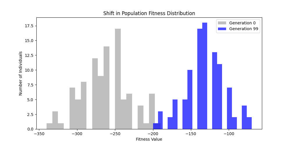
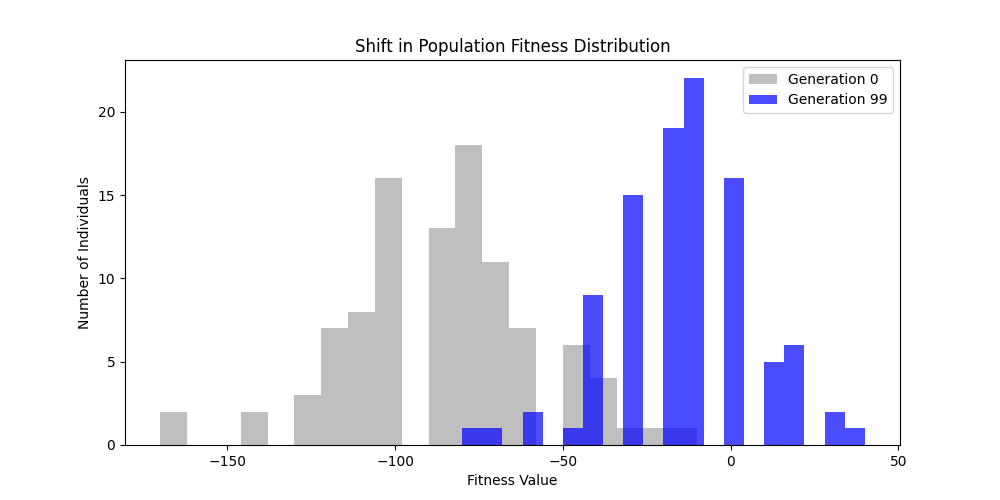
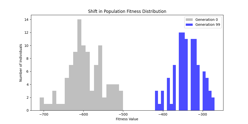
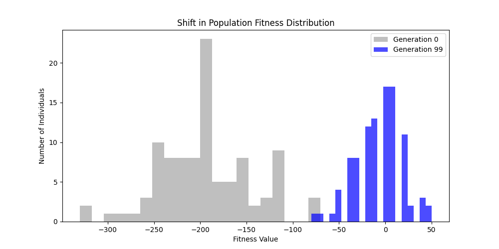
1. Fitness Functions

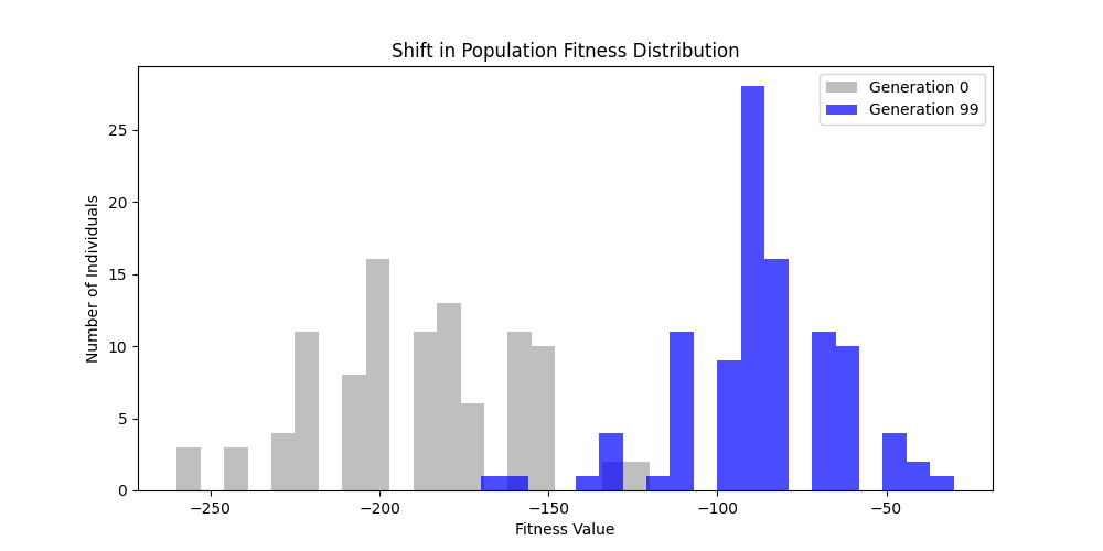
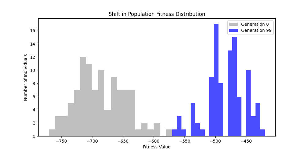
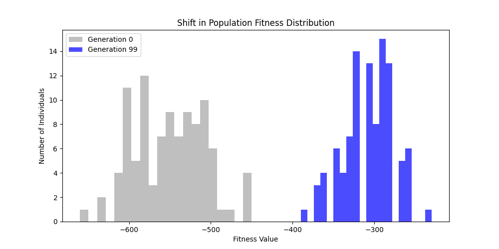
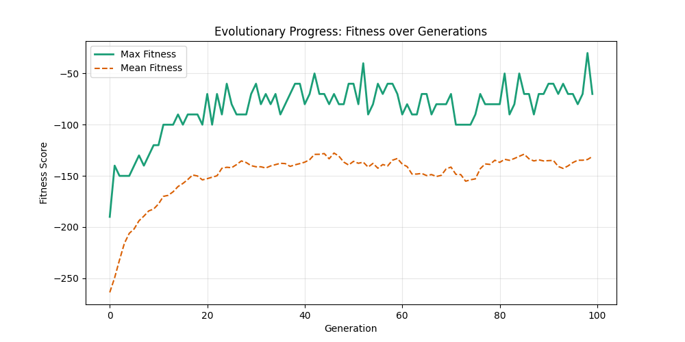
As defined previously, we have 2 functions: hard constraints (only viable individuals) vs soft constraints (penalty for invalid edges). We will try on small graph instances, in which a solution is guaranteed to exist, and compare the convergence speed and success rate of both approaches.

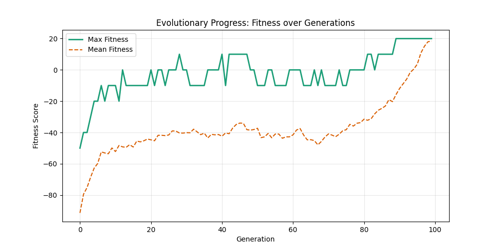
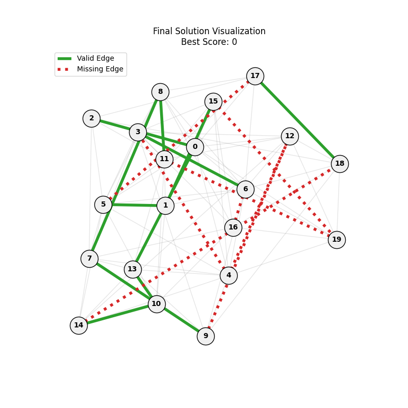
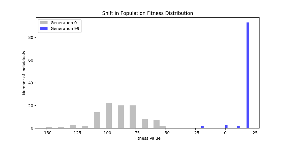
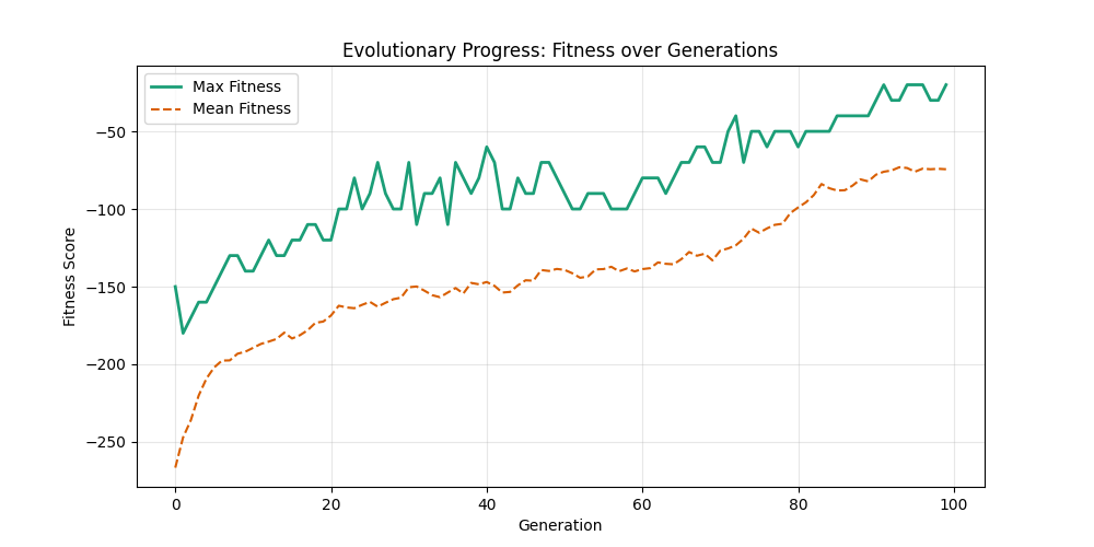
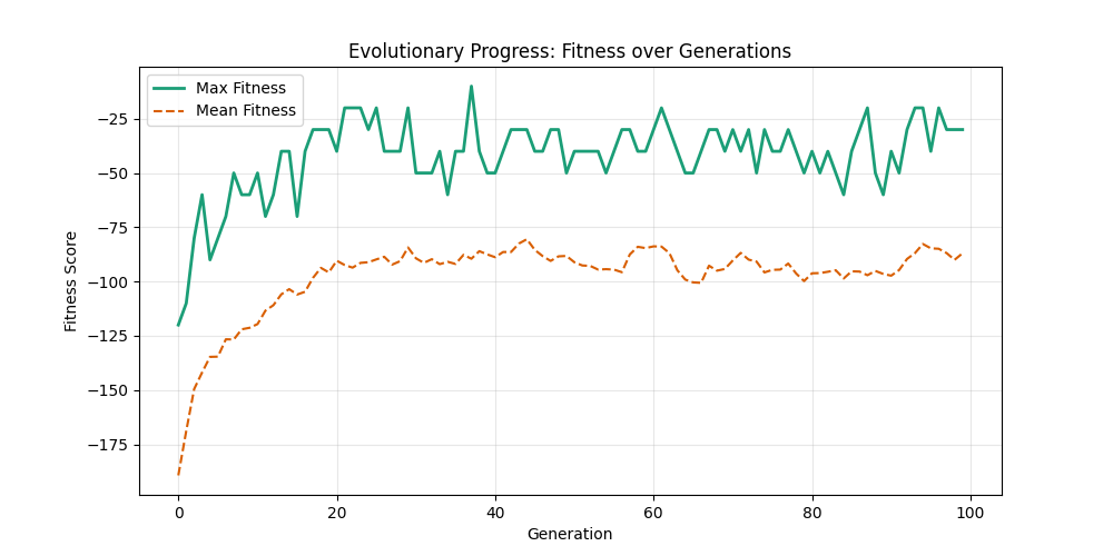
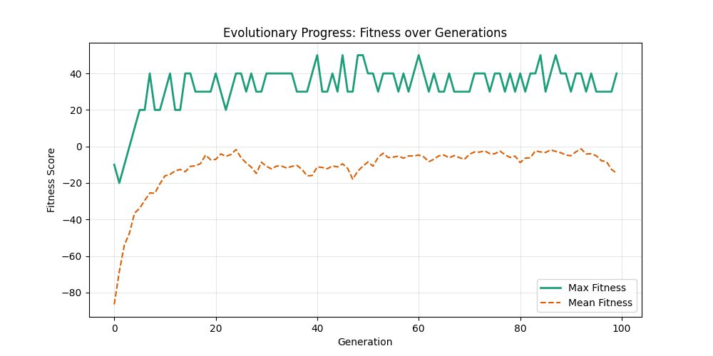
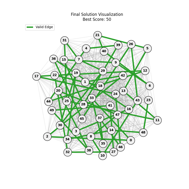
For each experiment and following the Albert-Barabasi model with n=20 nodes and m=4 edges per new node, over 100 generations with a population size of 100:

Soft Fitness	Hard Fitness

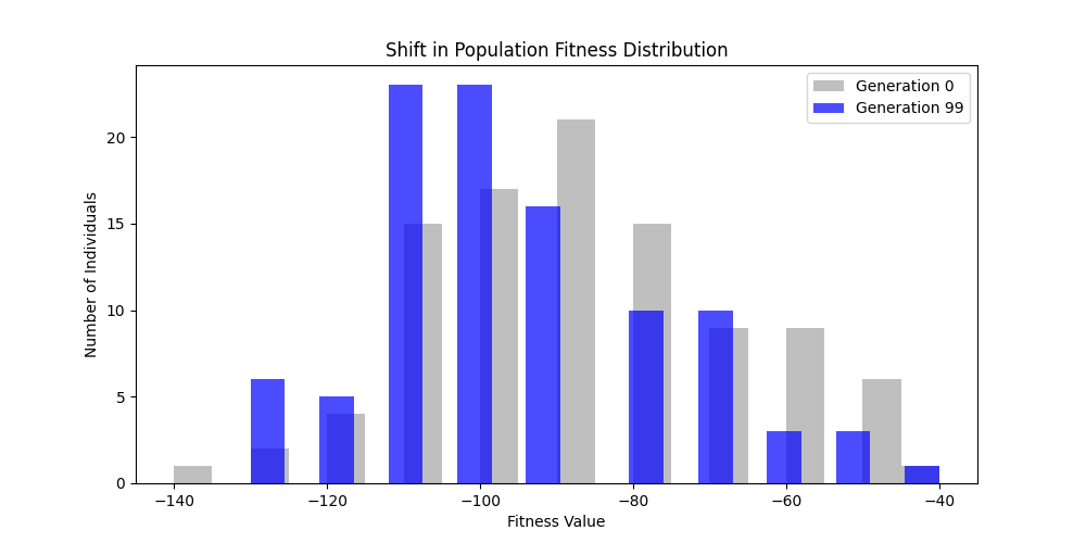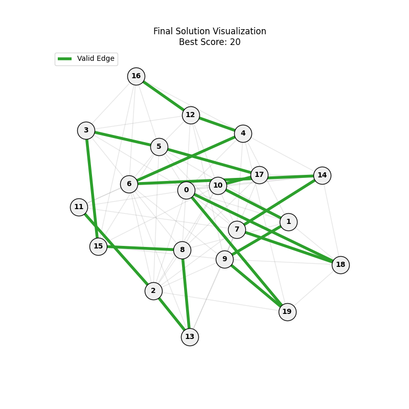
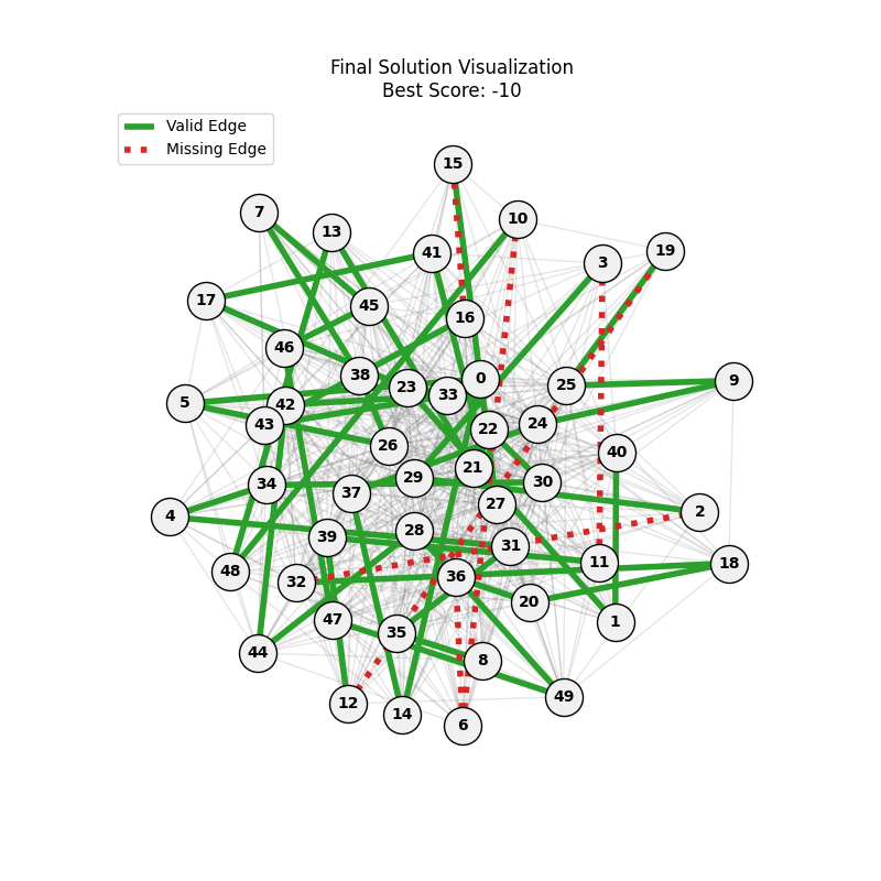
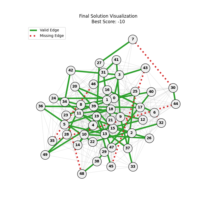
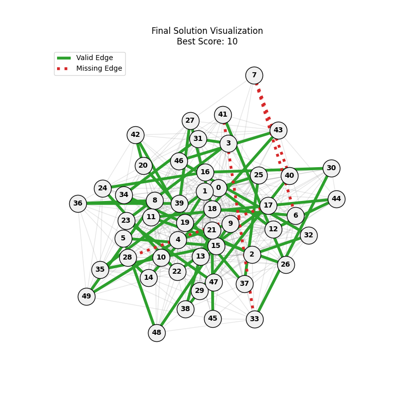
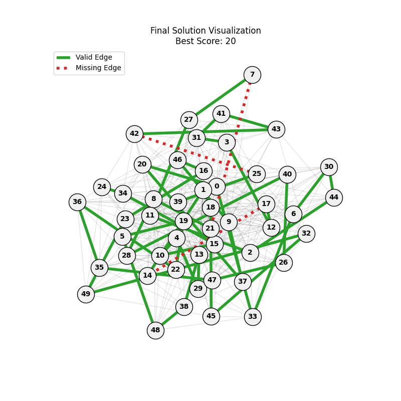
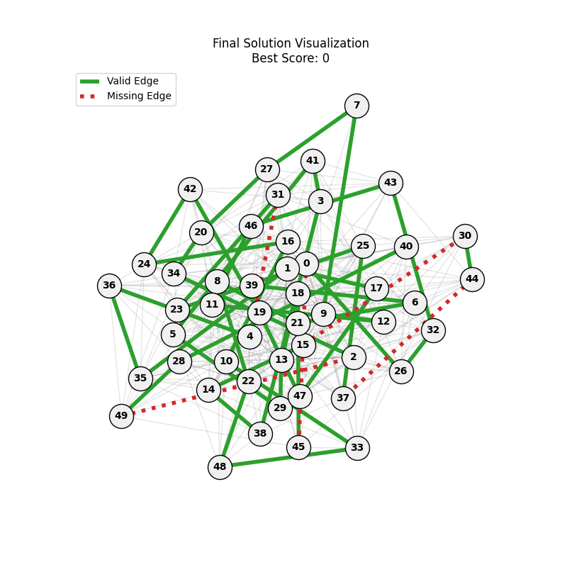
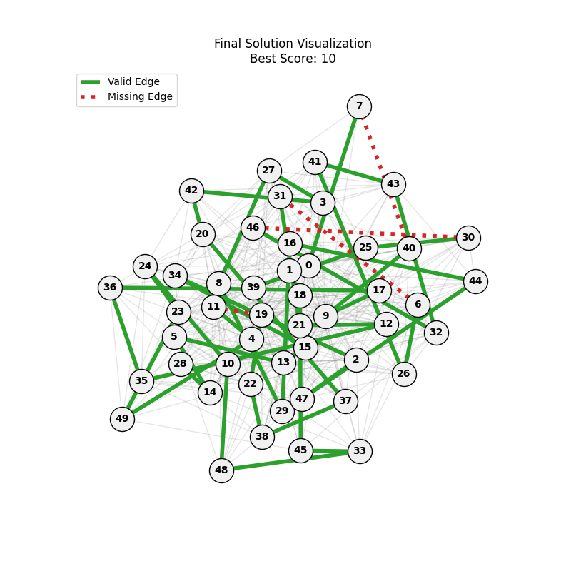
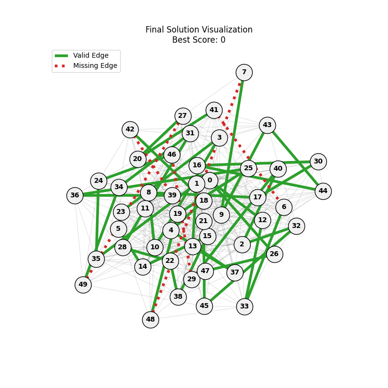
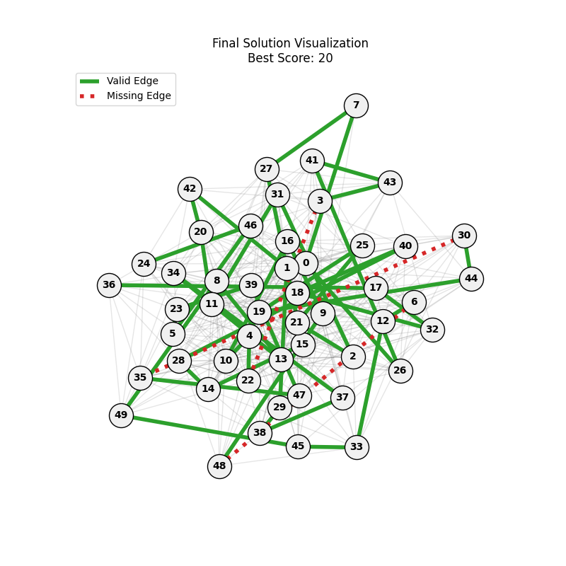
Noticing, since the problem statement is harsh (viability is only binary, and its NP hard to find a solution), we can not evolve a solution smoothly. However, for a small instance graph (size 20 with sufficient connectivity), both the soft function was able to find a solution at around Generation 80. Thus we will continue exploring with the soft function where there is more room for evolution.

2. Graph Types and Sizes

This is only to experiment on different problem sizes and structures, so different graph instances performances

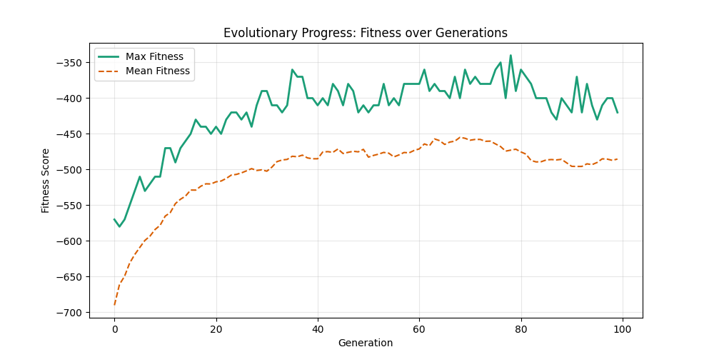
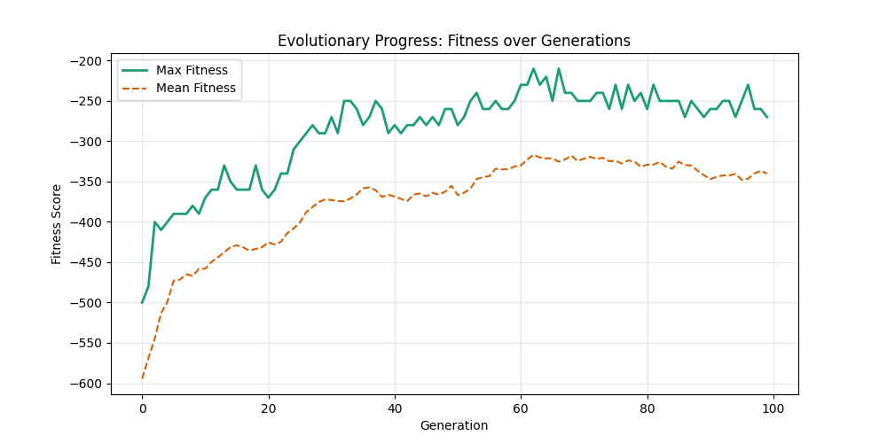
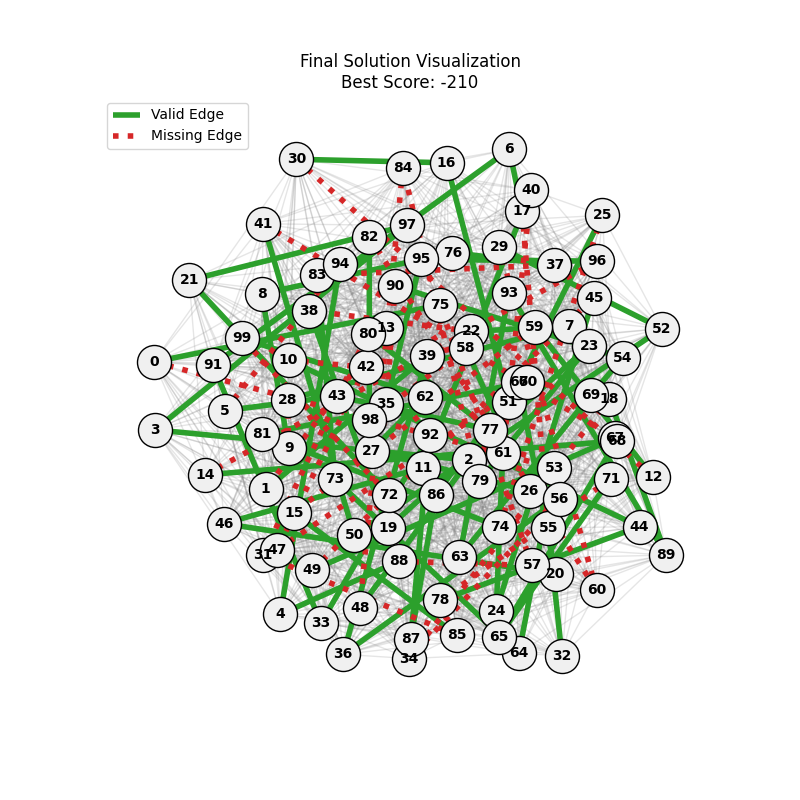
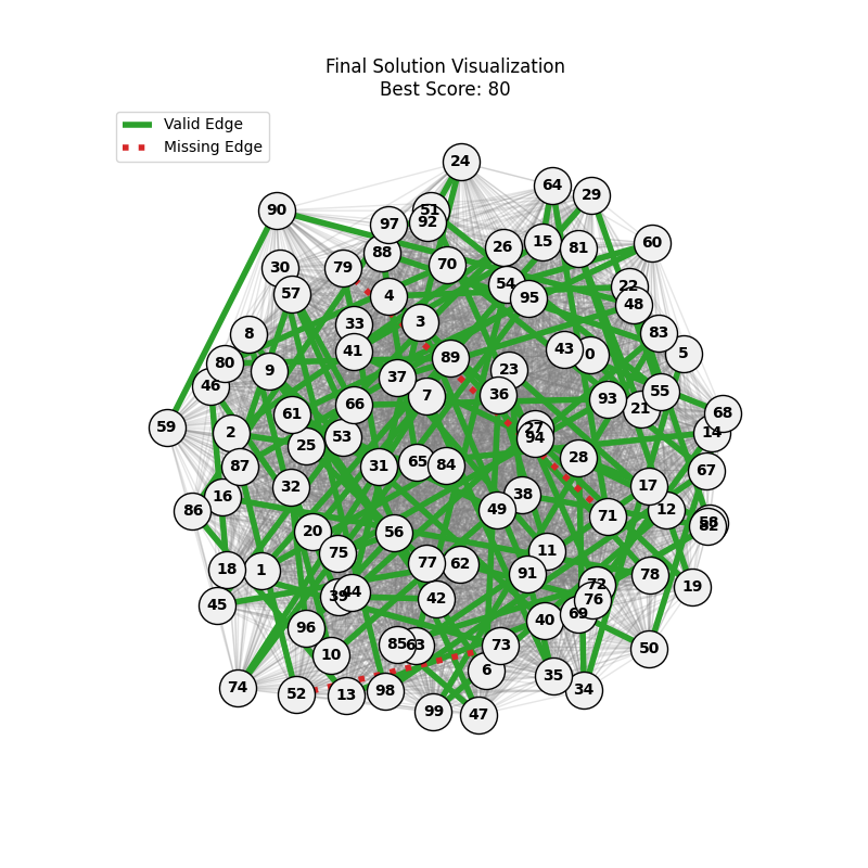
We will be experimenting on different graph types (Erdos-Renyi vs Albert-Barabasi) and sizes (n=50, 100) to observe the effect of graph structure on the GA’s performance. For each graph type and size, we will run the GA with the soft fitness function and record the convergence behavior.
Also note some other parameters:

erdos-renyi: p=0.3 and p=0.7 will be tested
albert-barabasi: m=10 and m=20 will be tested

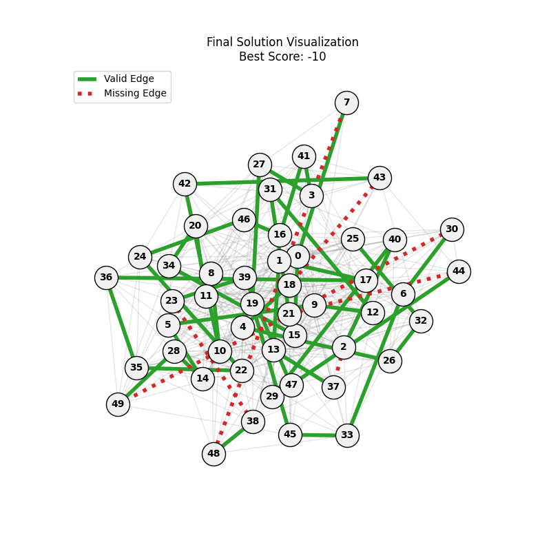
Starting with Albert-Barabasi graphs: | n=50, m=10 | n=50, m=20 | n=100, m=10 | n=100, m=20 | |———————–|———————–|–|–| | Fitness Evolution AB 50 | | Fitness Evolution AB 100 | | | Best Path AB 50 | | Best Path AB 100 | | | Population Distribution AB 50 | | Population Distribution AB 100 | |

We notice the following trends:

Increasing the number of edges per new node (m) generally improves the GA’s performance, as it increases the graph’s connectivity, making it easier to find Hamiltonian Paths.
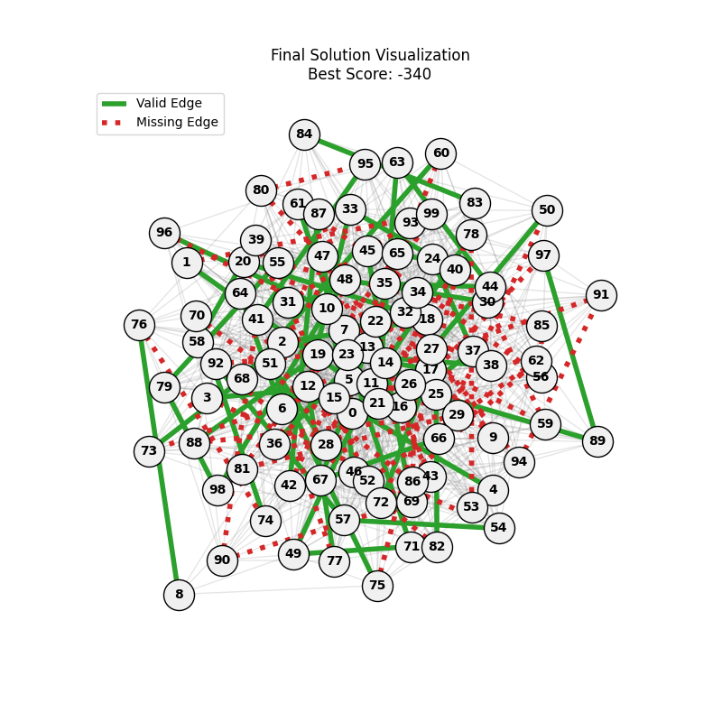
Larger graphs (n=100) pose more challenges, but with sufficient connectivity (m=20), the fitness still shows improvement over generations and becomes nearer to the optimal solution
For large sizes, the computation takes more time and the convergence is slower, in fact unlike the n=20 example previously, we could not at any case really find a full VALID hamiltonian path, but we could get very close to it (high fitness values) which is reflected in real life NP hard problems

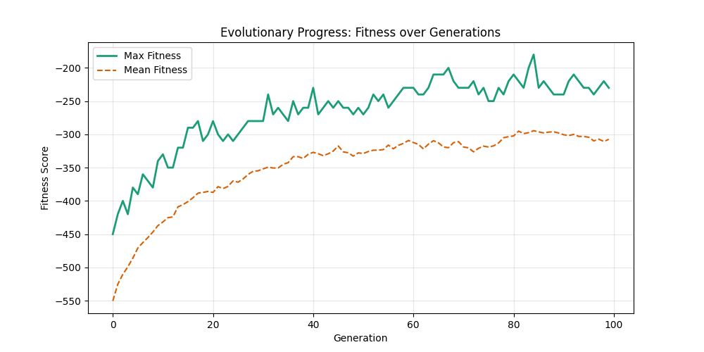
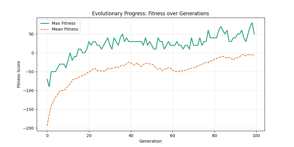
For Erdos-Renyi graphs: | n=50, p=0.3 | n=50, p=0.7 | n=100, p=0.3 | n=100, p=0.7 | |———————–|———————–|–|–| | Fitness Evolution ER 50 | | Fitness Evolution ER 100 | | | Best Path ER 50 | | Best Path ER 100 | | | | Population Distribution ER 50 | | Population Distribution ER 100 | |

Now random and scale-free graphs are not directly comparable as they have different parameters, but in general, we notice convergence faster in erdos-renyi, particulalry for highly connected graphs (p=0.7). Again, due to the more uniform distribution of edges, which provides more potential paths for the GA to explore.
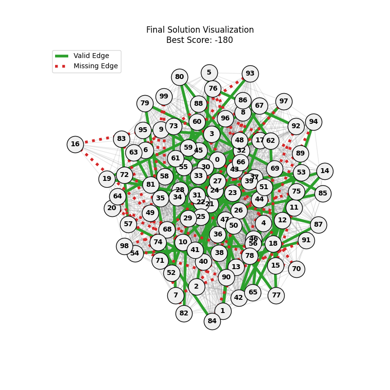
In fact, for n=50, the optimal solution was found around generation 100 since the graph was dense enough. For n=100, the GA struggled more, but still showed improvement in fitness over generations with a final solution near an optimal path.
In here, the size of the graph had a more pronounced effect, as the random nature of edge distribution in larger graphs made it harder to find Hamiltonian Paths compared to the scale-free graphs.

3. GA Hyperparameter Tuning

To perform a comprehensive hyperparamter tuning, we will be using GridSearchCV from scikit-learn to explore different combinations of key GA parameters:

Mutation Rate: [0.01, 0.05, 0.1]
Crossover Rate: [0.7, 0.8, 0.9]

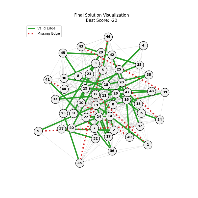
As for number of generations and population size, the higher they are, the better the results will be, but at the cost of computation time. Thus we will fix generations=100 and population size=100 for the tuning experiments on a n=50 m=10 scale free graph.

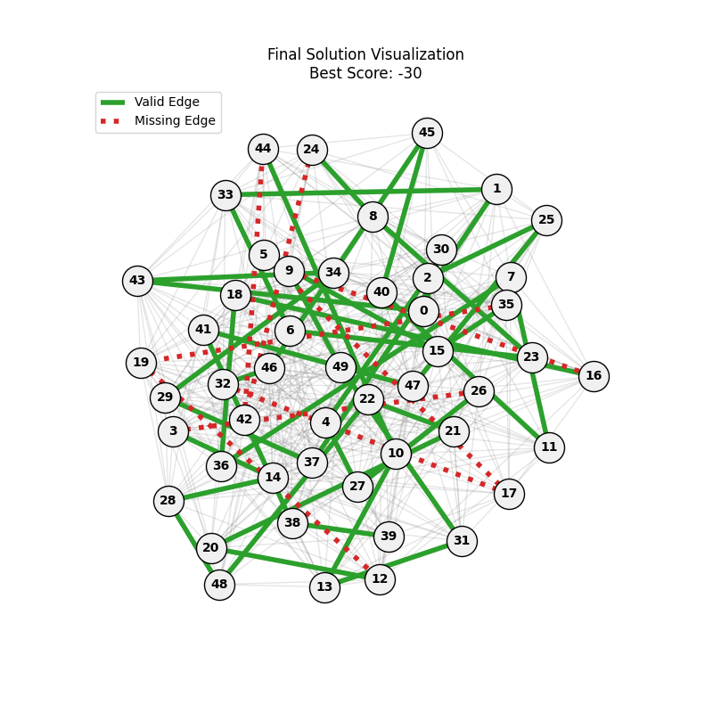
Hyperparameters	Fitness Evolution	Graph Best Path
mut=0.01, ox=0.7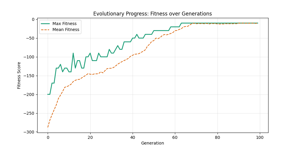
mut=0.01, ox=0.8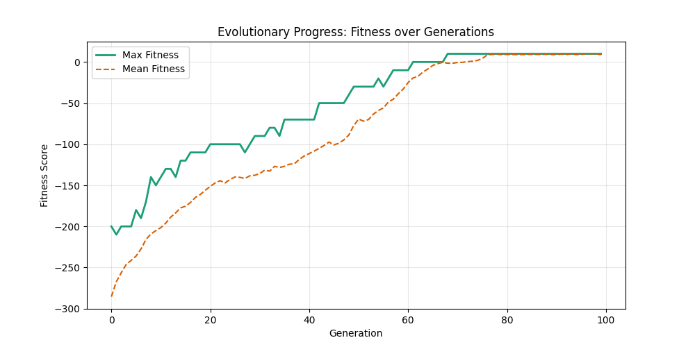
mut=0.01, ox=0.9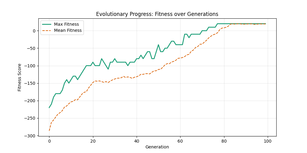
mut=0.05, ox=0.7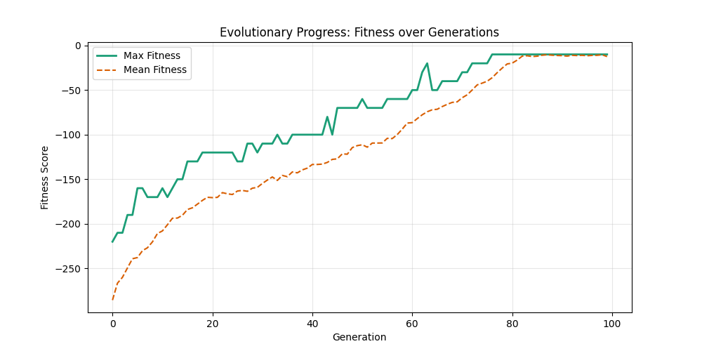
mut=0.05, ox=0.8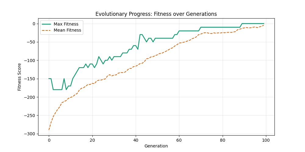
mut=0.05, ox=0.9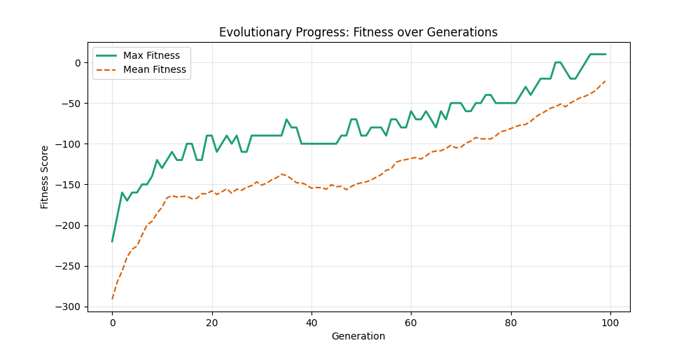
mut=0.1, ox=0.7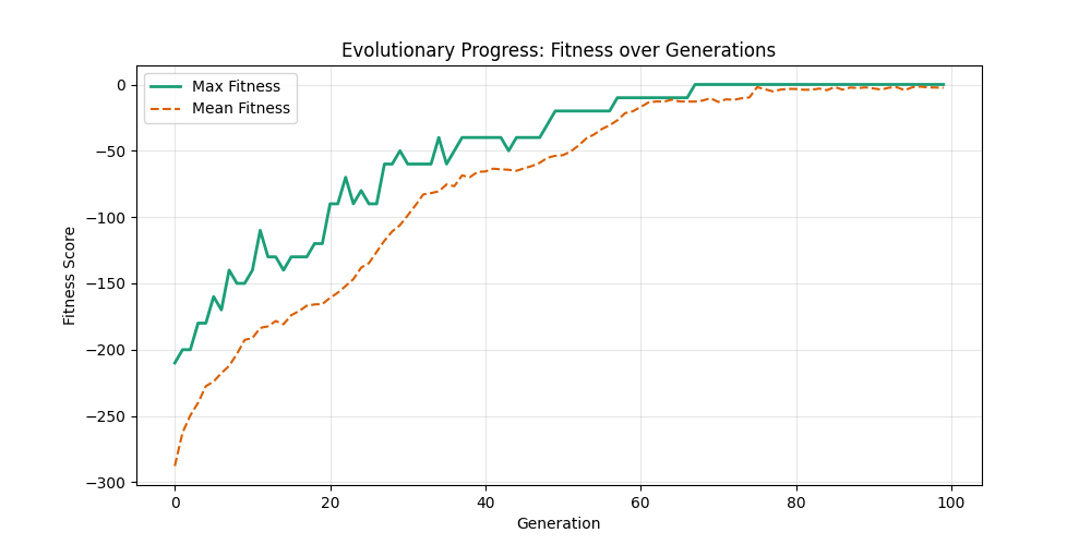
mut=0.1, ox=0.8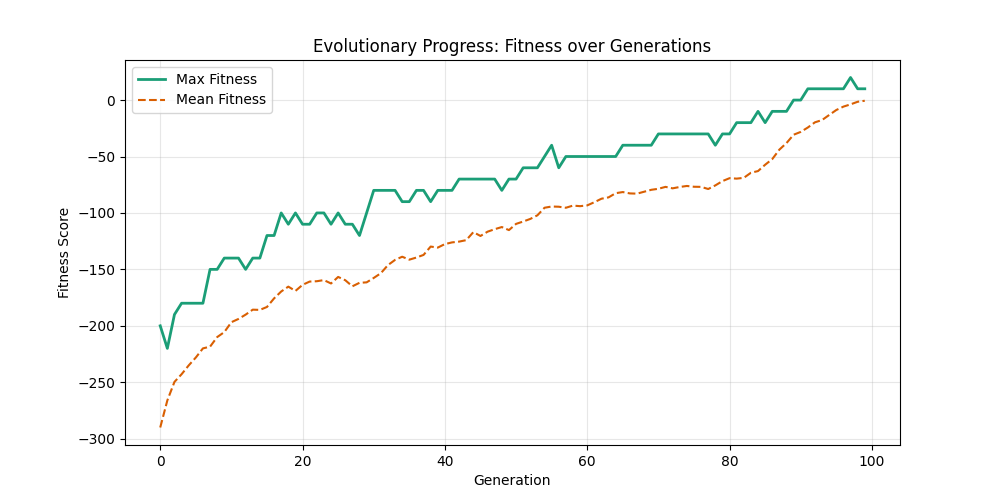
mut=0.1, ox=0.9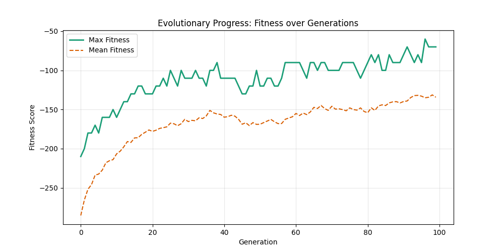

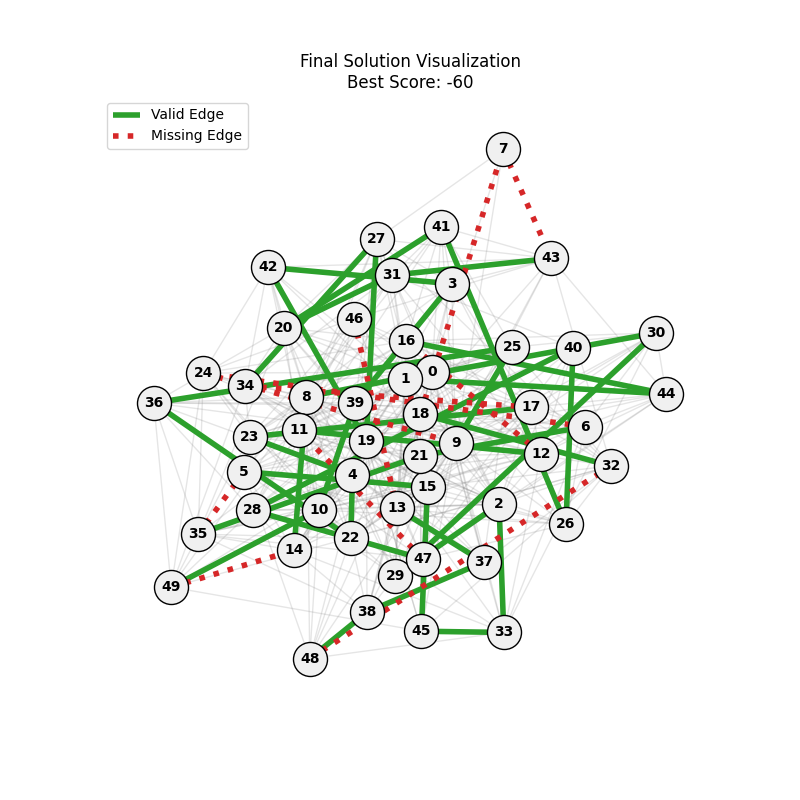We can concluse best scores at mutation rate=0.01 and cross-over rate=0.9 with 3 invalids only.

Genome Assembly Application

In a genome assembly context, the graph is constructed from DNA fragments (k-mers) as nodes, and edges represent overlaps between these k-mers. The goal is to find a Hamiltonian Path that visits each k-mer exactly once, effectively reconstructing the original DNA sequence from the fragments. This is obviously an open problem with no deterministic polynomial-time solution, hence we use metaheuristic methods like Genetic Algorithms to find near optimal solutions efficiently.

This problem is described in depth on another github repository: raysas/graph-genome-assembler

Hamiltonian Path Example

In order to apply this GA approach to genome assembly, it’s worth noting the differences on the graph structure level:

directed graph: order of k-mers matters, overlap CAA $\rightarrow$ AAT is correct, not the same as AAT $\rightarrow$ CAA (incorrect overlap)
unweighted but multiple nodes: the graph should be designed in a way that allows multiple identical k-mers to exist as separate nodes, since in real DNA sequences, certain k-mers can appear multiple times. We do not care for edge multiplicity, as we only need to know if there is an overlap or not (binary relationship)

This site is open source. Improve this page.